PV curves and loading margin

A PV curve shows how bus voltage changes as a power transfer increases. Its maximum loading point, or nose, defines the loading margin in megawatts. solve_pv_curve traces the curve and identifies whether the maximum is a smooth voltage-collapse point or is caused by an equipment limit.

The sink and source arguments use the endpoint definitions from transfer capability. These examples create cases in Python, but the calculation also accepts RAW, RAWX, and MATPOWER cases.

A feeder with a known collapse point

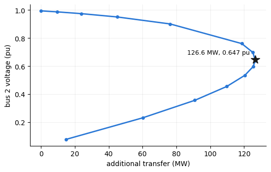
A lossless feeder with reactance \(X = 0.3\) pu supplies a load from a unit-voltage source. The load increases in the direction \((P_0, Q_0) = (1.0,\,0.2)\) pu. The maximum occurs at \(s^* = (\sqrt{P_0^2 + Q_0^2} - Q_0)\,/\,(2 X P_0^2)\), with load voltage \(\sqrt{1/2 - X Q}\) at the fold. The base case includes 10 MW in this direction. The remaining margin is 126.63 MW, and the nose voltage is 0.6465 pu.

import math

from gpf import (Bus, Branch, Generator, Load, GpfCase,
                 PfContinuationOptions, solve_pv_curve)


def build_feeder():
    """A two-bus feeder: unit-voltage source, X = 0.3 pu line, 10 MW base
    load at 0.98 power factor."""
    buses = [Bus(ibus=1, ide=3, baskv=230.0), Bus(ibus=2, ide=1, baskv=230.0)]
    gens = [Generator(ibus=1, machid="1", stat=1, pg=10.0, pt=500.0, pb=0.0,
                      vs=1.0, qt=9999.0, qb=-9999.0)]
    branches = [Branch(ibus=1, jbus=2, ckt="1", r=0.0, x=0.3, b=0.0, stat=1)]
    loads = [Load(ibus=2, loadid="1", pl=10.0, ql=2.0, stat=1)]
    return GpfCase(sbase=100.0, rev=33, basfrq=60.0, buses=buses,
                   generators=gens, branches=branches, loads=loads,
                   fixed_shunts=[], transformers=[], gen_costs=[])


feeder = build_feeder()

X, P0, Q0 = 0.3, 1.0, 0.2
s_star = (math.hypot(P0, Q0) - Q0) / (2 * X * P0**2)
(round(100 * (s_star - 0.1), 2), round(math.sqrt(0.5 - X * Q0 * s_star), 4))

(126.63, 0.6465)

Tracing the curve

solve_pv_curve increases the load at bus 2 at its initial power factor. This matches the load direction above. The result identifies a smooth fold at the calculated margin and voltage. It identifies bus 2 as the weak bus.

curve = solve_pv_curve(feeder, sink={2: 1.0})
i2 = list(curve.bus_ids).index(2)
{"nose_kind": curve.nose_kind, "nose_mw": round(curve.nose_mw, 2),
 "pinned": bool(curve.pinned), "weak_bus": curve.weak_bus,
 "nose_vm": round(float(curve.nose_vm[i2]), 4)}

{'nose_kind': 'fold',
 'nose_mw': 126.63,
 'pinned': True,
 'weak_bus': 2,
 'nose_vm': 0.6465}

The nose curve

The load-bus voltage decreases on the upper part of the curve. The trace passes the maximum loading point and continues on the lower part until it reaches the voltage limit. The marker shows the calculated nose.

import matplotlib.pyplot as plt

fig, ax = plt.subplots(figsize=(5.6, 3.6))
ax.plot(curve.lam_mw, curve.vm[:, i2], color="#2a78d6", lw=2,
        marker="o", ms=4)
ax.plot(curve.nose_mw, float(curve.nose_vm[i2]), marker="*", ms=13,
        color="#1a1a19", ls="none")
ax.annotate(f"{curve.nose_mw:.1f} MW, {float(curve.nose_vm[i2]):.3f} pu",
            xy=(curve.nose_mw, float(curve.nose_vm[i2])),
            xytext=(-8, 8), textcoords="offset points", ha="right", fontsize=9)
ax.set_xlabel("additional transfer (MW)")
ax.set_ylabel("bus 2 voltage (pu)")
ax.grid(alpha=0.3, lw=0.5)
for side in ("top", "right"):
    ax.spines[side].set_visible(False)
fig.tight_layout()

A reactive limit moves the maximum

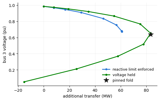
A second system has a generator that regulates its bus at 1.02 pu and has a 30 Mvar reactive-power limit. The default limit_mode="enforce" setting applies this limit. The generator reaches the limit, the bus voltage is no longer regulated, and the maximum falls to 60.9 MW. The result identifies this maximum as limit-induced. If the calculation ignores the limit, the curve reaches a smooth fold at 83.5 MW.

def build_system():
    """Slack, a regulating generator (1.02 pu, 30 Mvar ceiling), and a
    30 MW load bus behind an X = 0.35 pu line."""
    buses = [Bus(ibus=1, ide=3, baskv=230.0), Bus(ibus=2, ide=2, baskv=230.0),
             Bus(ibus=3, ide=1, baskv=230.0)]
    gens = [Generator(ibus=1, machid="1", stat=1, pg=0.0, pt=500.0, pb=0.0,
                      vs=1.0, qt=9999.0, qb=-9999.0),
            Generator(ibus=2, machid="1", stat=1, pg=30.0, pt=500.0, pb=0.0,
                      vs=1.02, qt=30.0, qb=-900.0)]
    branches = [Branch(ibus=1, jbus=2, ckt="1", r=0.01, x=0.10, b=0.0, stat=1),
                Branch(ibus=2, jbus=3, ckt="1", r=0.03, x=0.35, b=0.0, stat=1)]
    loads = [Load(ibus=3, loadid="1", pl=30.0, ql=6.0, stat=1)]
    return GpfCase(sbase=100.0, rev=33, basfrq=60.0, buses=buses,
                   generators=gens, branches=branches, loads=loads,
                   fixed_shunts=[], transformers=[], gen_costs=[])


system = build_system()
limited = solve_pv_curve(system, sink={3: 1.0})
held = solve_pv_curve(system, sink={3: 1.0},
                      options=PfContinuationOptions(limit_mode="hold"))
{"enforced": (limited.nose_kind, round(limited.nose_mw, 1)),
 "voltage_held": (held.nose_kind, round(held.nose_mw, 1))}

{'enforced': ('limit_induced', 60.9), 'voltage_held': ('fold', 83.5)}

The two curves

The plot compares both traces at the load bus. The voltage-held curve reaches a smooth maximum. The enforced curve reaches the generator limit first. regime_change marks the points where the equipment status changes. The limit-induced maximum is an estimate, so pinned is False.

i3 = list(limited.bus_ids).index(3)
fig, ax = plt.subplots(figsize=(5.6, 3.6))
ax.plot(limited.lam_mw, limited.vm[:, i3], color="#2a78d6", lw=2,
        marker="o", ms=4, label="reactive limit enforced")
ax.plot(held.lam_mw, held.vm[:, i3], color="#008300", lw=2,
        marker="o", ms=4, label="voltage held")
ax.plot(held.nose_mw, float(held.nose_vm[i3]), marker="*", ms=13,
        color="#1a1a19", ls="none", label="pinned fold")
ax.set_xlabel("additional transfer (MW)")
ax.set_ylabel("bus 3 voltage (pu)")
ax.legend(frameon=False, fontsize=9)
ax.grid(alpha=0.3, lw=0.5)
for side in ("top", "right"):
    ax.spines[side].set_visible(False)
fig.tight_layout()

(bool(limited.pinned), bool(held.pinned), int(limited.regime_change[1]))

(False, True, 1)

Reviewing weak locations

The result identifies the bus most associated with the reported limit. Use this location to prioritize engineering review.

{"weak_bus": held.weak_bus}

{'weak_bus': 3}

Choosing the endpoints

The sink and source arguments accept a bus number or a {bus: weight} mapping. If you omit source, the swing bus supplies the transfer. If you name a source, generation increases at that location. The selected endpoints therefore affect the margin. A nearby source raises the enforced maximum from 60.9 MW to 62.6 MW. A weighted sink that assigns 30 percent of the load growth to the generator bus raises it to 86.2 MW.

sourced = solve_pv_curve(system, sink={3: 1.0}, source={2: 1.0})
weighted = solve_pv_curve(system, sink={2: 0.3, 3: 0.7})
{"sourced": (sourced.nose_kind, round(sourced.nose_mw, 1)),
 "weighted_sink": (weighted.nose_kind, round(weighted.nose_mw, 1))}

{'sourced': ('limit_induced', 62.6), 'weighted_sink': ('limit_induced', 86.2)}

Run the same calculation from the command line with gpf study pv CASE --sink BUS. Use --limit-mode hold to trace the voltage-held curve. Transfer capability explains the available endpoint forms.