QV curves and reactive margin

A QV curve shows the reactive power required to maintain a selected bus voltage. The lowest point on the curve defines the reactive margin at that bus. solve_qv_curve traces the curve and reports the margin and the voltage at the lowest point.

These examples create cases in Python, but the calculation also accepts RAW, RAWX, and MATPOWER cases. PV curves explains the related active power and voltage calculation.

A feeder with a known bottom

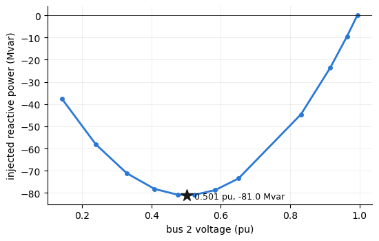
This example uses the lossless feeder from PV curves. For line reactance \(X\), fixed load \(P\), and initial reactive load \(Q_0\), the reactive margin is \((1/4 - X^2 P^2)/X - Q_0\). The lowest-point voltage is \(\sqrt{1/4 + X^2 P^2}\). All values in these equations use per unit. For \(X = 0.3\), \(P = 0.1\), and \(Q_0 = 0.02\), the margin is 81.03 Mvar and the lowest-point voltage is 0.5009 pu.

import math

from gpf import (Bus, Branch, DCOPFError, Generator, Load, GpfCase,
                 PfContinuationOptions, solve_qv_curve)


def build_feeder():
    """A two-bus feeder: unit-voltage source, X = 0.3 pu line, 10 MW base
    load at 0.98 power factor."""
    buses = [Bus(ibus=1, ide=3, baskv=230.0), Bus(ibus=2, ide=1, baskv=230.0)]
    gens = [Generator(ibus=1, machid="1", stat=1, pg=10.0, pt=500.0, pb=0.0,
                      vs=1.0, qt=9999.0, qb=-9999.0)]
    branches = [Branch(ibus=1, jbus=2, ckt="1", r=0.0, x=0.3, b=0.0, stat=1)]
    loads = [Load(ibus=2, loadid="1", pl=10.0, ql=2.0, stat=1)]
    return GpfCase(sbase=100.0, rev=33, basfrq=60.0, buses=buses,
                   generators=gens, branches=branches, loads=loads,
                   fixed_shunts=[], transformers=[], gen_costs=[])


feeder = build_feeder()

X, P, Q0 = 0.3, 0.1, 0.02
(round(100 * ((0.25 - X**2 * P**2) / X - Q0), 2),
 round(math.sqrt(0.25 + X**2 * P**2), 4))

(81.03, 0.5009)

Tracing the curve

solve_qv_curve traces the curve at bus 2. The result identifies a smooth fold at the calculated margin and voltage.

curve = solve_qv_curve(feeder, 2)
{"nose_kind": curve.nose_kind, "margin_mvar": round(curve.margin_mvar, 2),
 "pinned": bool(curve.pinned), "v_bottom": round(curve.v_bottom, 4)}

{'nose_kind': 'fold', 'margin_mvar': 81.03, 'pinned': True, 'v_bottom': 0.5009}

The curve

The plot shows voltage on the horizontal axis and reactive-power injection on the vertical axis. The curve minimum gives the reactive margin below zero. The calculation selects points along the curve, so the voltage intervals are not uniform.

import matplotlib.pyplot as plt

fig, ax = plt.subplots(figsize=(5.6, 3.6))
ax.plot(curve.v, curve.q_inj_mvar, color="#2a78d6", lw=2, marker="o", ms=4)
ax.plot(curve.v_bottom, -curve.margin_mvar, marker="*", ms=13,
        color="#1a1a19", ls="none")
ax.annotate(f"{curve.v_bottom:.3f} pu, {-curve.margin_mvar:.1f} Mvar",
            xy=(curve.v_bottom, -curve.margin_mvar),
            xytext=(8, -4), textcoords="offset points", fontsize=9)
ax.axhline(0.0, color="#1a1a19", lw=0.6)
ax.set_xlabel("bus 2 voltage (pu)")
ax.set_ylabel("injected reactive power (Mvar)")
ax.grid(alpha=0.3, lw=0.5)
for side in ("top", "right"):
    ax.spines[side].set_visible(False)
fig.tight_layout()

A reactive limit lowers the margin

The second system from PV curves has a generator that regulates its bus at 1.02 pu and has a 30 Mvar reactive-power limit. The default limit_mode="enforce" setting applies the limit. The generator reaches the limit and stops regulating the bus voltage. This reduces the reactive margin to 48.3 Mvar. If the calculation ignores the limit, the margin is 63.8 Mvar. Both curves reach a smooth fold.

def build_system():
    """Slack, a regulating generator (1.02 pu, 30 Mvar ceiling), and a
    30 MW load bus behind an X = 0.35 pu line."""
    buses = [Bus(ibus=1, ide=3, baskv=230.0), Bus(ibus=2, ide=2, baskv=230.0),
             Bus(ibus=3, ide=1, baskv=230.0)]
    gens = [Generator(ibus=1, machid="1", stat=1, pg=0.0, pt=500.0, pb=0.0,
                      vs=1.0, qt=9999.0, qb=-9999.0),
            Generator(ibus=2, machid="1", stat=1, pg=30.0, pt=500.0, pb=0.0,
                      vs=1.02, qt=30.0, qb=-900.0)]
    branches = [Branch(ibus=1, jbus=2, ckt="1", r=0.01, x=0.10, b=0.0, stat=1),
                Branch(ibus=2, jbus=3, ckt="1", r=0.03, x=0.35, b=0.0, stat=1)]
    loads = [Load(ibus=3, loadid="1", pl=30.0, ql=6.0, stat=1)]
    return GpfCase(sbase=100.0, rev=33, basfrq=60.0, buses=buses,
                   generators=gens, branches=branches, loads=loads,
                   fixed_shunts=[], transformers=[], gen_costs=[])


system = build_system()
limited = solve_qv_curve(system, 3)
held = solve_qv_curve(system, 3,
                      options=PfContinuationOptions(limit_mode="hold"))
{"enforced": (limited.nose_kind, round(limited.margin_mvar, 1)),
 "voltage_held": (held.nose_kind, round(held.margin_mvar, 1))}

{'enforced': ('fold', 48.3), 'voltage_held': ('fold', 63.8)}

Voltage-controlled buses

A regulated bus cannot change voltage while its regulator maintains the setpoint. With enforced limits, the trace starts at 1.02 pu. It moves downward after the generator reaches its reactive-power limit and stops regulating the bus. With limit_mode="hold", the regulator does not release the bus, so the calculation rejects the trace. The calculation also rejects a trace at the swing bus because its voltage is fixed.

at_machine = solve_qv_curve(system, 2)
(round(float(at_machine.v[0]), 4), round(float(at_machine.v.min()), 4))

(1.02, 0.5663)

try:
    solve_qv_curve(system, 2,
                   options=PfContinuationOptions(limit_mode="hold"))
except DCOPFError as err:
    message = str(err)
message

'the voltage at bus 2 is held by a regulator that never released over the trace, so the QV direction has no free Q row; enforce (finite) reactive limits or study another bus'

Screening several buses

A multi-bus screen traces one curve for each selected bus. The bus with the smallest reactive margin is the weakest. This example adds bus 4 behind another 0.25 pu of reactance and places a 10 MW load there. The remote bus has a margin of 28.7 Mvar, compared with 41.9 Mvar at bus 3. Both curves reach a smooth fold.

outer = build_system()
outer.buses.append(Bus(ibus=4, ide=1, baskv=230.0))
outer.branches.append(Branch(ibus=3, jbus=4, ckt="1", r=0.02, x=0.25,
                             b=0.0, stat=1))
outer.loads.append(Load(ibus=4, loadid="1", pl=10.0, ql=2.0, stat=1))

{bus: round(solve_qv_curve(outer, bus).margin_mvar, 1) for bus in (3, 4)}

{3: 41.9, 4: 28.7}

Run the same calculation from the command line with gpf study qv CASE --bus BUS. Repeat --bus to trace more than one bus. Use --limit-mode hold to trace the voltage-held curve. PV curves explains the related result fields.